Uniswap: An Options Market

Introduction

The goal of this article is to show how Uniswap is not only a decentralized exchange for buying and selling digital assets but also a type of options market. The one sided marketplace introduces implied volatility over historical, or expected volatility, as a better metric to judge a Uniswap pool’s performance from the perspective of liquidity providers. I will focus on Uniswap V2 for the sake of simplicity but the logic of the argument presented in this article can be extended to Uniswap V3 because of its similarity to V2.

Currently the most often touted metric of a pool’s performance is its yield from trading fees. Marketers of Uniswap pools like to display a pool’s two to three digit yield as an incentive for investors to provide liquidity in a pool. However, this is the wrong metric to judge a pool’s performance since it does not take into account the volatility of the underlying assets of the pool and therefore the expected impermanent loss.

What is an Option?

To better understand the similarity of a Uniswap liquidity pool to an option’s marketplace, one must first understand the characteristics of an option in traditional financial markets.

An option is a financial contract that gives the buyer the right but not the obligation to purchase or sell an asset at a predetermined price, the strike price, prior to or at an expiration date.

The possibility of the option gaining substantial value as the underlying asset price moves into the money is referred to as optionality and is the reason why an option’s price is an irrelevant metric when judging the potential of an option as an investment.

Rather, it is the probability of the option expiring in the money which is the most important metric. This probability, after taking some assumptions into consideration, can be measured with the volatility of the underlying asset.

How are Options Priced?

In traditional financial markets the Black Scholes Model is the most common model used to price traditional option contracts. The explanation of the Black Scholes Model is beyond the scope of this article, therefore to summarize its contributions, the Black Scholes Model identifies the characteristics of the underlying asset and option contract that drive the price of the option.

Its most significant inference is that the volatility of the underlying asset is the most important factor in determining the price of the option. That is because the greater the volatility, the higher the likelihood that the option will expire in the money (be profitable upon exercise).

Hence the proper way to price an option is in terms of its implied volatility, that is the volatility the option’s current premium implies the market expects. Since, assuming that there is no arbitrage opportunity, at this volatility the option’s premium does not convey any advantage to the seller or buyer of the option. That is, under the no arbitrage principle of asset valuation, whatever profit the buyer of the option could make will be on average negated by the premium she paid for the option. Just as whatever profit the option seller can make will be on average negated by the loss she will experience when the option expires in the money

A Simple Options Trading Strategy

Given that under the no arbitrage principle the premium one pays or receives for the option grants no possibility of being consistently profitable over time, the assumption a profit seeking trader makes is that the option’s premium is too high or too low. That is, the implied volatility of the option is either too high or too low relative to the actual volatility the underlying asset will realize throughout the life of the option. Or in other words, the probability the market estimates that the option will expire in the money is too high or too low to what the actual probability is.

One estimate of this actual volatility is typically the historical volatility of the asset. Of course there are many other ways to estimate this actual volatility, such as having greater insight about a company’s future earning reports, or better prediction ability of macroeconomic or geopolitical events relative to the market’s expectations. The point being that estimating implied volatility relative to actual volatility is the most important metric to keep track of when trading options.

Delta Hedging

Given that the most important metric in determining the price of an option is the asset’s expected volatility, it stands to reason that a trader may seek to solely trade the volatility implied by the option’s premium.

By focusing on only trading volatility, she can increase the consistency of her returns since she becomes indifferent to the option expiring in the money or out of the money. As long as the realized volatility is lower than the implied volatility at which she sold the option, or vice versa if she bought the option, she will come out ahead with a profit. How she accomplishes this is by hedging away the effects of the underlying asset’s price movements on the option though a strategy called delta hedging.

The delta of an option is the change in price of the option with respect to change in price of the underlying asset. This number can be calculated using the Black Scholes Model. The point of calculating this number is to buy or short the underlying asset in quantities that match the delta of the option in the opposite direction. That is to hedge away the effects of price variation from the underlying asset on the option. That way the option trader remains mostly exposed to the volatility of the option.

However, as the price of the underlying moves in one direction the delta of the option also changes, this change can become substantial so that the option’s delta is no longer properly hedged. This risk is referred to as gamma exposure, which is the second derivative of the option with respect to the price of the underlying asset in the Black Scholes Model.

Dynamic Hedging

Therefore, in order to account for the gamma exposure, option traders engage in what is called dynamic hedging. That is they constantly re-hedge their delta exposure every time there are significant changes in the underlying price. After a certain period of time, they calculate the delta of the option again and adjust their hedge with the underlying asset to match the new delta. This eventually results in a situation where as the price of the underlying asset moves toward one direction, the option trader has to buy more of the underlying asset to maintain delta neutrality.

The goal of dynamic hedging is therefore to replicate the delta returns of the option in the opposite direction of the option trader’s position to hedge away the exposure to directional moves in the underlying asset. Thus leaving the option trader exposed only to the volatility of the underlying asset, e.g. vega risk as defined in the Black Scholes Model.

Given that in traditional financial markets implied volatility is often higher than realized volatility, selling volatility is usually a profitable strategy. This is akin to selling insurance in more conventional markets. People tend to overestimate the likelihood of detrimental events, hence they overpay for the safety blanket of insurance.

Uniswap’s Dynamic Hedging

If you are a keen observer and familiar with the dynamics of the Uniswap algorithm, you will realize that the Uniswap smart contract is dynamically hedging the pool whenever there is a movement in the price of the underlying assets.As the price moves in one direction, Uniswap increases the reserves quantity of one asset and decreases the other. Uniswap’s algorithm is therefore replicating the negative delta of long put options on the assets it holds as reserves through dynamic hedging. Uniswap accomplishes dynamic hedging by incentivizing external traders to adjust its reserve quantities through price discrepancies with other exchanges. If we were to imagine an Uniswap pool holding put options on its reserves, its algorithm is dynamically hedging the value of its options in terms of its reserve assets, as the price of its reserve assets change with respect to each other.

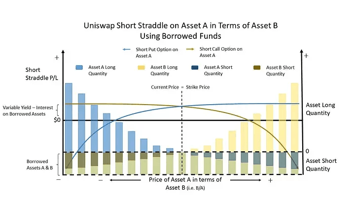
In the chart above as the price of asset A falls, the Uniswap pool increases its long exposure to asset A to counter the increasingly higher rate of change in the value of a hypothetical long put option on asset A and vice versa as the price of asset A rises. However, since both assets are priced in terms of each other, as the price of asset A falls, it means the price of asset B is rising relative to asset A. Therefore, the Uniswap pool must decrease its long exposure to asset B to properly hedge the lower rate of change in the value of a hypothetical put option on asset B that is priced in terms of asset A.

Uniswap’s Embedded Options

Since Uniswap is dynamically hedging an exposure to hypothetical long put options on its reserves, then it is essentially always taking the opposite trade of long put options on its reserves.

Therefore, an Uniswap pool, at any point in time, is holding short put options on its reserves. We can therefore think of Uniswap pools as holding embedded short put options, which liquidity providers expose themselves to when they add liquidity to a pool.

The difference between Uniswap’s embedded options and traditional options is that traditional options have an expiration date, a capped delta (e.g. for stock options it is typically 100 because contracts are written for only 100 shares), a one time premium, and a strike price that can be different from the current price. An Uniswap embedded option is perpetual, its strike price at the time of sale is always the current price (i.e. it’s always sold at the money), its premiums payments are variable and paid in perpetuity, and it is written for an infinite number of units of the asset. That means its delta can increase to infinity.

The Straddle

In traditional financial markets a straddle is an options portfolio that an investor can purchase to expose himself to the volatility of an asset. This strategy consists of buying a call and put option on the same underlying with the same strike price and expiration at the same time.

The straddle buyer pays the premiums of the options but he realizes his profit as the price of the underlying moves significantly in either direction. He is profitable when the difference between the underlying and strike is greater than the combined premiums he paid for both option contracts. This is therefore a long volatility position that is indifferent of market direction. As the volatility of the underlying asset increases, the higher the likelihood his position will turn positive.

On the other side of this trade is a straddle seller. That is someone who sells a call and put option on the same underlying with the same strike price and expiration. His return profile is the opposite of that of the straddle buyer. Whereas the straddle buyer benefits as volatility goes, a straddle seller benefits when volatility decreases and the price of the underlying remains the same until expiration. The straddle seller’s profit is the premiums of the option he sold minus the exercisable value of the options at expiration, if one of them expires in the money. A straddle seller is short volatility.

Uniswap Liquidity Provision: The Perpetual Short Straddle

We established earlier than an Uniswap pool is at all times holding short put positions on its reserve assets. However, since each asset is priced in terms of the other asset, one of the short puts can also be thought of as a short call on the other asset.

In the picture above the short put on asset B can be thought of as a short call on asset A. That is because in order to replicate the short call on asset A we have to lower our exposure to asset A. Since we can’t short asset A directly, we instead reduce our exposure by selling increasing quantities of asset A. Since asset A is priced in terms of asset B, we are increasing our exposure to asset B.

Therefore, an Uniswap pool can be thought of as holding a short put and short call on one of its reserve assets — priced in terms of the other asset in the pool.

If you wanted to more clearly represent the similarity of an Uniswap liquidity position to a short straddle, one could borrow both reserve assets and provide them as liquidity to the pool. In that case the requirement to first have both assets disappears, and the diminishment of one asset’s quantity does indeed represent a short position. In addition, an interest rate exposure is introduced since the borrowed funds will accrue interest and must therefore be subtracted from the yield from trading fees.

Therefore, an Uniswap liquidity provision position is nothing more than a short straddle with the characteristics of it being perpetual (no theta/time risk), variable continuous premium from trading fees, and sold with strike prices equal to the current market price. In other words, a swap of volatility or gamma risk for a perpetual stream of payments from trading fees.

A Better Measure of an Uniswap Pool’s Return

Given that we can think of Uniswap liquidity pools as a marketplace for selling straddles, a better way to judge the potential of liquidity provision in a pool as an investment is the implied volatility of the pool. It is a metric I explained how to calculate in the previous article.

Just like with traditional option markets, if the implied volatility of an Uniswap pool’s pair is higher than the historical volatility of the pair, or whatever other measure of actual expected volatility a trader may use, providing liquidity to the pool is considered positive EV. This because the yields from trading fees will on average be greater than the impermanent loss the liquidity provider will experience.

However, if the pool’s implied volatility is lower than a trader’s measure of actual expected volatility of the underlying pair, then the pool’s liquidity provision return has negative expected value.

To better illustrate this point, let’s take an example. First remember our formula for implied volatility from the previous article.

Now, suppose there’s a pool paying a yield of 20% APY, and a mean return of 0% on the reserve pair. That is, the pair is not expected to change in value in the long term, although it is expected to experience volatility. Assuming that we will provide liquidity for one year, we can deduce the implied volatility as follows,

We calculated the implied volatility the market predicts to be approximately 126%. Now remember our formula for expected impermanent loss including the pool yield from trading fees from the previous article.

Our implied volatility calculation indicates that if the actual volatility the market experiences over the same time period is approximately 126%, we can expect to experience an impermanent loss of 0% after including the yield from trading fees, assuming the yield stays constant.

Then, suppose we expected the actual volatility to be lower, at let’s say 100%. Then our expected return for such a pool using our formula for expected impermanent loss including yield from trading fees from the previous article would be the following

Our expected return is positive at approximately 7.79%. However, had we expect the actual volatility to be greater, such as 150%, then our expected return would’ve been the following

Our expected return is negative at approximately -7.8%.

As we can see from the example, whenever implied volatility is higher than historical or expected volatility, providing liquidity to an Uniswap pool provides positive expected return.

If the implied volatility is lower than the historical or expected volatility, the return becomes negative. Therefore, implied volatility relative to whatever metric of expected volatility we use is a better determinate of EV than pool yield alone.

Conclusion

In this article I explained how an Uniswap pool has embedded options and is therefore a type of options market for selling straddles. Hence, implied volatility of the pool, as indicated by the pool’s yields, compared to the pool’s underlying pair’s historical volatility is a better measure of the pool’s potential as an investment.

In the next article, I’ll explain how throughout most of its history Uniswap liquidity pools have expressed an implied volatility that is lower than the historical volatility of the underlying pairs. Therefore, for most of its history, Uniswap pools have been negative EV to LP into.

I’ll explain why this is the case and provide a solution to this problem. In a follow on article, I’ll provide a way to separate the embedded call and put options from an Uniswap liquidity pool so that liquidity providers can better hedge their risk exposures.