Total Returns and Impermanent Loss in Uniswap V2

Intro to Return Profiles and IL

In the previous article, I described how Uniswap V2 operates, with a particular focus on how CFMMs replicate market impact events in CLOBs. To summarize, the substitution of one token for another happens at a sublinear rate, leading to a change in the ratio of the reserve quantities held within the pool. This imbalance affects the value of the LP’s position. Therefore, any calculation of total return for a liquidity provider must take into account the change in value of the pool’s reserves.

First we must separate returns into two parts: returns due to trading fees and returns due to price variation.

Trading Fees

Uniswap uses the product of the reserves to determine quotes for traders. Fortunately, when calculating the square root of this product, the geometric mean, we can measure the growth of the pool’s reserves.

Since liquidity shares from the pool increase only when LPs add additional liquidity to the pool, the growth of the geometric mean of the reserves due to trading fees belongs completely to LPs. Therefore, assuming there is no change in the ratio of the reserves of the pool, that is price is constant, the value of the LP’s stake grows at an exponential rate from trading fees. Assuming the initial value of a LP’s stake is C and the geometric mean grows at a constant rate, α, the total value at any time t can be calculated thusly,

Where, α, a constant, is the growth rate of the pool’s reserves from trading fees per unit of time t. We use Euler’s number, e, because we are assuming continuous compounding of the trading fees, since all fees are always reinvested in the pool immediately because they are collected as additional reserves. To derive the return using this formula simply set C = 1 and subtract 1.

Price Variation

In Uniswap V2 the reserves are assumed to be equal in value to each other. Therefore, the price quoted by the pool can be measured as the ratio of the reserves. Since this ratio changes when trades occur, an LP’s stake fluctuates along with this ratio. The following function gives the value of the reserves held in the pool.

Where V is the value of the liquidity in the pool dependent on price, and x and y are the quantities of tokens X and Y, respectively, held in reserve. However, we do not want to have a function depending on the values of x and y.

In order to simplify this equation we can take advantage of the fact that Uniswap V2 uses the product of the reserves to quote prices during trades, which must remain a constant, excluding trading fees, and finding the square root to arrive at the geometric mean.

Where x and y are the reserve quantities of tokens X and Y, respectively, and L is the geometric mean of the reserve quantities, the liquidity invariant.

And we also take advantage of the fact that in Uniswap the price is measured as the ratio of the two reserve quantities.

Therefore it follows that

Substituting the values of x and y into the equation for the geometric mean of the reserve quantities, we can derive

Therefore, using the original function for the value of the reserves held in the pool as a function of price and the definitions x and y in terms of L and p,

To derive the return of the stake in the liquidity pool set the initial p = 1, which means the initial value of the liquidity stake is 2L. Then calculate the return from 2L.

The returns of the liquidity pool with respect to price variation move at a sublinear rate with respect to price. For example, a 1,184% price increase corresponds to roughly a 250% appreciation in the value of the liquidity pool. Conversely, a 74% decline in the price corresponds to about a 50% decline in the value of the liquidity pool. This relationship is obvious since the return grows as the square root of price. Calculating the first derivative with respect to price yields

That is, the rate of growth of the return with respect to price trends to 0 (no change) at an increasingly diminishing sublinear rate as price moves to infinity. Meanwhile, it maintains a less than linear change until a 75% decline from the price, at which liquidity was provided has occurred (p = 0.25 makes the denominator equal to 1). That is, decreases in price are less than 1 for 1 until price is at 25% of the original price. After that point, the curve approaches negative infinity at a faster than linear rate.

Total Return

Before we derive the total return we must first state the formula for the value of the stake in the liquidity pool taking into account price variation and trading fees. That is combining the two formulas above.

Where α is the growth rate of the geometric mean of the pool’s reserves, the liquidity invariant, per unit of time t.

Now to measure the return from t = 0 to t = 1 we would use the following formula

Which after simplification becomes

If we define P as the price ratio of p at any t from p at t = 0, then we can generalize the return formula as follows for any time t,

We can now plot the graphs of the total returns of the liquidity provider’s stake at different growth rates of the pool’s reserves from trading fees as price varies.

As can be seen above, trading fees can have a substantial effect on the returns of the liquidity pool. If the growth rate of the pool is high enough, the returns of the liquidity pool can be greater than the returns of price alone. For example, if α = 20%, then a price change of 20% corresponds to a return of 100%. However, due to the return’s square root relationship with price, the effect of a high α decreases as price deviates from the original price at which liquidity was provided.

For example, for a 519% change in price, the return of the pool is only 350%. Despite the growth from trading fees, the derivative of the return function with respect to price is still tending towards 0 (no change) as price goes to infinity, while maintaining its sublinear relationship until a 75% price decline has occurred.

Impermanent Loss

Impermanent loss is a misnomer because it is not an actual loss liquidity providers experience but rather an opportunity cost. Impermanent loss is the difference between the value of the liquidity provider’s stake in the pool and the value of the same stake had it not been supplied as liquidity to the pool, excluding trading fees earned by the liquidity pool.

Due to the sublinear effect trading activity has on the pool’s reserves, as the reserve ratio (price) changes, the performance of the stake supplied as liquidity to the pool (excluding trading fees) always underperforms the stake not invested in the pool. The underperformance increases in significance the greater the price change. Since the goal of measuring impermanent loss is to estimate this opportunity cost, it always ignores the trading fees earned by the liquidity pool.

The formula for the impermanent loss is the following

where k is a number from 0 to infinity that represents the change in price (the reserve ratio) from the time liquidity was provided to the pool.

Impermanent Loss Derivation

To derive the impermanent loss function, we have to first define a formula for the value of the liquidity stake had it not been supplied to the liquidity pool. First create a future price variable called p’ which is equal to p*k where p is the initial price at which liquidity is provided and k is a number within 0 and infinity.

Then, using the formula defined above for the value of the stake in the liquidity pool but using p’ instead, we can derive the following,

Therefore the formula for the value of the liquidity stake had it not been invested in the liquidity pool is

Now, we plug in p’ in the formula for the value of the stake that is invested in the pool to derive the same formula as a function of k (the value of the stake invested in the liquidity pool in the next timestep).

Finally, to derive the impermanent loss we subtract the difference of the two values of the stake as a percentage of the stake that was not invested in the liquidity pool.

As you can see, impermanent loss (IL) increases as the price deviates from the original price at which liquidity was provided. It is called impermanent because if the price ever reverts back to the original price at which liquidity was provided, the loss disappears.

Why is Impermanent Loss Important

Impermanent loss is an important metric because it lets us estimate the potential underperformance of liquidity provision relative to holding funds outside of a liquidity pool. However, impermanent loss cannot be the only metric one takes into consideration since a liquidity pool also earns trading fees.

Therefore, one must add trading fees to the return function of the funds in the liquidity pool, to measure the actual performance of a liquidity pool.

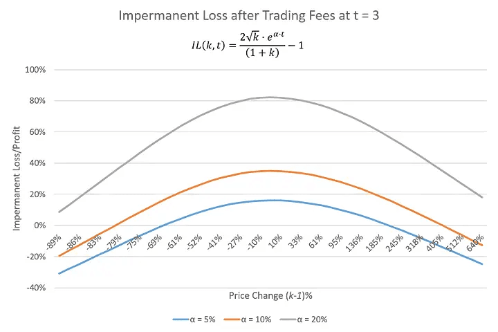
Adding Trading Fees to Impermanent Loss

To add trading fees, we simply substitute the formula for the value of the stake in the liquidity pool above including trading fees for the value of the stake in the liquidity pool excluding trading fees in the impermanent loss equation,

After some simplification we get the following,

As you can see from above, trading fees can substantially remediate underperformance of IL or even outperform at dramatic price changes.

Conclusion

Returns in Uniswap V2’s liquidity pool move at a sublinear rate with respect to price while price is above 25% of the value at which liquidity was provided. That is, as price increases, the return increases at a progressively reduced rate, however, when price decreases, the returns also decrease at a reduced rate until they cross the 25% threshold. After that point, the relationship becomes greater than linear with respect to price. However, trading fees can add substantial upside while maintaining the sublinear relationship with price. Unfortunately, the effect of trading fees on returns decrease as price deviates further away from the original price at which liquidity was provided. This is due to the square root relationship between returns and price for funds inside Uniswap’s liquidity pool.

Although CFMMs like Uniswap use the name market maker, their returns profiles are uniquely different to that of traditional firms. Traditional market makers hedge price variation and limit their returns to the bid ask spread of the markets they make. However, liquidity provision in Uniswap carries a substantial amount of inventory risk at all times. The risk is unhedged product the LP provider is carrying in her book. Therefore, when investing in an Uniswap liquidity pool, a rational LP is betting that the trading fees she collects will be greater than the losses from price declining and ideally greater than the underperformance from IL. However, this exposure to losses from price declining negatively skews the potential returns of liquidity pools.

In the next article I’ll introduce a way to improve the risk adjusted returns of LPing by hedging away market risk and driving returns through the accumulation of trading fees.