Optimizing Liquidity Provision: Hedging Market Risk in Uniswap V2

Introduction to Hedging Risk

In the previous article I explained how to calculate returns from liquidity provisioning in Uniswap V2. I showed how liquidity provision carries a substantial amount of market risk, which although benefits the liquidity provider when prices move up its at an ever decreasing rate, while the risks increase substantially as the prices drop. The exposure to market risk increases the variability of returns substantially to LPs, which although might still lead to outperformances in the short term when there is high volume, can be further optimized if market risk were hedged.

In this article, I’ll demonstrate a way to hedge market risk while LPing and prove how hedging leads to better risk adjusted returns that can be magnified through leverage.

Hedged Liquidity Provision

In an unhedged liquidity provision, as we’ve seen in the previous article, the value of the stake in the liquidity pool is determined by the following function

where α is the growth rate of the liquidity pool from trading fees in terms of units of time t, x and y are the quantities of the assets provided to the liquidity pool, p is the price of asset X in terms of Y at t = 0, L is the geometric mean of quantities x and y, a constant, and k is a number between 0 and infinity that represents the change of price, p. As you can see the value of this function is solely determined by the price, p. In order to hedge the price therefore we must take the opposite position of the asset that is priced in terms of y. That is we must short asset X.

We could achieve such a short position by borrowing asset X using asset Y as collateral. Then, the hedged portfolio becomes

where θ is a number that represents the percentage of the liquidity position that is being shorted. Typically between 0 and 1 but could be greater than 1 if we seek to obtain a net short position. We also added the interest rate, r, on the loan for the short measured per units of time t. The sign next to x is negative while the sign next to y is positive because when we open the short, we borrow x (hence we are short x) and sell it for y (hence are long y). Hence we are short x in terms of y.

Unfortunately, creating a short position usually requires margin. That is, the borrower must put up additional collateral to cover the short in case of losses on the short position. Therefore, short positions are typically overcollateralized to ensure there are always enough funds to cover the liquidation. Hence we add parameter φ, which is the collateralization ratio we wish to use for the asset we are borrowing. That is if φ is 70% then the amount borrowed must equal 70% of the collateral. Therefore φ is always a number greater than 0 but less than 1. Since most trading platforms will usually have a collateralization ratio for borrowed assets upon which they force liquidations, one must always choose a value for φ that is greater than the liquidation limit for the lending platform.

We also added parameter ω, which represents the percentage of liquidity provided in the pool due to the collateralization ratio. Since, if we need to overcollateralize the short position, there is less capital available to provide as liquidity. This parameter ω is not chosen by the liquidity provider, it is rather dependent on the values of θ and φ.

One thing to note is that ω will normally be less than or equal to 1. That is because θ will normally be in the range [0, 1). θ is the percentage of our entire liquidity position that we wish to short. θ is divided by two because we can only create a short from half of our entire capital available for liquidity provision. The value in parenthesis

is the collateral to debt ratio of the lending platform where we borrow tokens to create the short position, which is always positive because 0 < φ < 1. That is how much collateral has to be posted to create a short position. That ratio multiplied by θ and divided by two always creates a value greater than 0. Therefore, if we are not hedging our liquidity position, then we will provide our entire capital as liquidity (ω = 1). If we are hedging our liquidity position, then we will provide less than our entire capital as liquidity (ω < 1).

Since the value of x, y, L, and p have the following relationships,

We can define the hedged portfolio as follows,

Now to derive the return function we simply subtract and divide by the value of the liquidity provided at t = 0.

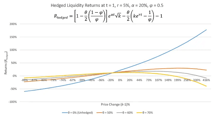
Which after simplification and expressing ω in terms of θ and φ, becomes

Setting the values of θ to 0.6 and φ to 0.5, which implies an ω of 0.7, we graph below the returns of the portfolio for different levels of α at t = 1

One thing to note is that since φ in the example above is 0.5, assuming that the the short position must never become greater than 90% of the collateral, we will either have to close the position or rebalance and decrease the hedge when the price increases by 80% to avoid liquidation. Therefore, the scenarios in the right of the chart, where the returns nosedive will be avoided by hedging. If we constantly rebalance the portfolio, the hedge will always be readjusting so that returns continue to increase with increases in price. The same can be done when prices decrease to avoid negative P&L. To do this one must increase the hedge as price decreases, although the effect of price declines are less significant.

The LP would have to make a judgement call on whether to change her hedge with price delta if she wishes to remain market neutral.

Lower Variability of Returns

The advantage of separating market risk from the returns of liquidity provision is the exposure to a different type of return profile. That is the return profile of a market maker. The return profile of a market maker is quite different than that of a spot trader. Even though an unhedged LP has lower return variability than a spot position in the underlying tokens of the liquidity pool, unless there’s a large price decline, the hedged LP will have even lower return variability. This phenomenon becomes apparent when analyzing the first derivative, with respect to price, of the return functions for hedged and unhedged liquidity provision.

When finding the difference between the two derivatives, we obtain

As mentioned earlier, the value of ω will always be less than 1. Therefore, the first derivative of the return of unhedged liquidity provision will always be greater than that of the hedged liquidity provision. Therefore, the variability of the returns of unhedged liquidity provision will always be greater than those of hedged liquidity provision. This is more clearly visible when looking at the range of the returns for unhedged and hedged liquidity provision.

The range of returns for unhedged liquidity provision is significantly greater than that of hedged liquidity provision assuming the same pool growth rate, α, and loan interest rate, r, even for different hedging hedging percentages, θ, at a collateral to debt rate of 2 (φ = 0.5).

Delta Neutrality

In the previous section we calculated the first derivative of the return function with respect to changes in price. The first derivative of a valuation formula is also called the delta of a portfolio, since it measures the change in returns for every change in price. Looking again at the equation of the delta of hedged liquidity provision and stating ω in terms of θ and φ, we can see that it is possible for the delta to become zero for certain values of θ, which we can choose at any time.

We do not need to focus on φ because it is typically determined by the lending platform where one borrows tokens to create the hedge, therefore, it is given as a constant.

If delta becomes zero then we are completely hedged for small changes in price. This is known as delta neutrality. It’s a strategy used by market makers to remain impervious to changes in market price and derive returns solely from market making. Of course, after large enough price deviations, we would have to readjust our θ to become delta neutral again.

To find the correct θ, we simply set the function to 0 and solve for θ.

Which yields

Since delta neutrality is measured from the time we open the position, we can assume k = 1 and t = 0. Therefore, at any given time to maintain delta neutrality θ must be

For example, assuming φ = 0.5, then θ must always be 2/3. Then ω is 2/3 meaning we should only be providing 2/3 of our available capital as liquidity and an amount equal to 1/3 of our capital as a hedge (θ/2).

For example, assuming α and r are 0, holding such a portfolio would sustain a loss of 1.33% if prices rise 44% or if they decline 36%. Without the hedge, the portfolio would suffer a loss of 20% if prices decline 36% and a gain of 20% if prices rise 44%.

To maintain delta neutrality after a significant price deviation, as in the case of a price rise of 44% or fall of 36%, the portfolio would have to be rebalanced to have an amount equal to 1/3 of the available capital as a hedge and 2/3 as liquidity provided in the pool.

Based on the table above, a liquidity provider would rebalance his portfolio every time price moves 20% up or down or if he wants to lower hedging costs rebalance when prices move 50% up or down.

Higher Sharpe Ratios

The Sharpe ratio is a measure of risk adjusted returns. It is calculated by dividing the expected difference of a portfolio’s return and the risk free rate of return divided by the standard deviation of the portfolio’s returns.

Where R_p and R_f are the portfolio’s rate of return and risk free rate of return respectively, and σ_p is the standard deviation of the portfolio’s returns (volatility). The Sharpe ratio provides the excess return over the risk free rate of return for every unit of risk (volatility) taken in the portfolio. Therefore, it can be thought of as a measure of risk adjusted returns.

A portfolio with a higher Sharpe ratio, despite lower returns, is preferable than one with a lower Sharpe ratio but higher returns. That is because the higher Sharpe ratio portfolio can be leveraged to increase the risk to match that of the lower Sharpe ratio portfolio and thus increase the return to higher levels than those of the lower Sharpe ratio portfolio.

For example, although delta neutral liquidity provision has lower returns than unhedged liquidity provision, the lower variability of the returns lead to a higher Sharpe Ratio, despite the lower absolute returns. Therefore, a leveraged delta neutral liquidity provision portfolio can have substantially higher returns than an unhedged liquidity provision portfolio.

Below are the Sharpe ratios of a delta neutral liquidity provision portfolio and a non hedged liquidity provision portfolio after a Monte Carlo simulation of 10,000 runs for a liquidity pool with different levels of growth (α), different volatilities and returns for the underlying pair of the liquidity pool, and different rebalancing strategies to achieve delta neutrality or restart the position in the unhedged portfolio (rebalancing every week and every month).

The instances where the Sharpe ratio of the delta neutral liquidity provision portfolio (hedging) was higher is highlighted in yellow. The risk free rate of return was assumed to be zero for the sake of simplicity. We also assumed a φ of 0.5 and therefore a θ of 1/3 to achieve delta neutrality.

As you can see in the tables above, the portfolio’s Sharpe ratio improves as alpha and the rebalancing period increase and worsens as volatility and returns in the underlying increase. However, the improvement from higher levels of α and rebalancing are much greater than the degradation from higher volatility and returns in the underlying.

For example, in the last table above, a hedged liquidity provision portfolio in a pool where the underlying is growing at 400% a year with a 100% annualized volatility (e.g. ETH/USD), that is rebalanced weekly, will have a Sharpe ratio (4.16) almost five times higher (4.84x) than that the unhedged liquidity provision portfolio (0.86).

That means returns of the hedged liquidity portfolio are almost five times higher than the unhedged liquidity portfolio, if the portfolio is leveraged enough to match the volatility. On the other hand under more stable levels of α (e.g. 20%), hedged liquidity provision outperforms only in periods of low volatility, with substantial outperformance in periods of low returns.

Leveraged Liquidity Provision

Given the higher Sharpe ratios of delta neutral liquidity provision a liquidity provider will be tempted to increase leverage in the strategy to more efficiently deploy capital. However, the increase in leverage comes at a cost of higher interest payments in loans to finance the higher leverage. This requires an update to the return calculation of hedged liquidity provision, to account for the interest accrued on the borrowed sums. All it amounts to is increasing the return by the leverage ratio and subtracting the additional interest accrued on the borrowed sums. Below we provide such formula.

Where f represents the equity to total assets rate (e.g. 20% means 20% is equity, 80% is borrowed sums, therefore a leverage ratio of 5). Therefore, the above formula can be stated more explicitly as

The first derivative of such a portfolio is simply the first derivative of the unleveraged portfolio multiplied by the leverage ratio.

Therefore, achieving delta neutrality (make the first derivative with respect to price zero) is the same process as for the non leveraged portfolio.

Conclusion

Hedging lowers the volatility of returns of liquidity provision substantially without compromising total returns as much and therefore accomplishes higher Sharpe ratios.

The higher Sharpe ratios allow for higher returns through more efficient use of capital. In this article, I assumed hedging was accomplished through loans on decentralized exchanges, but such loans can also be obtained from other sources. Closing the position requires selling the quantities to pay off the loans and accrued interest. Other trading expenses such as market impact and trading fees were not taken into account in this article.

In the following article, I’ll describe the similarities between liquidity provision and volatility trades in traditional derivatives markets. I will then propose my thesis that Uniswap V2 is a derivatives exchange for selling volatility.