Liquidity Provision at Any Strike Price Under Risk Neutral Pricing

Introduction to Long Gamma Strikes

In a previous article I modeled the performance of a liquidity provider in a CFMM such as Uniswap V2 providing liquidity at the current price, under the assumption of Geometric Brownian Motion. A common assumption made when modeling financial asset prices in quantitative finance.

In this article, I will generalize the model for providing liquidity at any price under the risk neutral pricing assumption, often used for pricing derivatives. This new model will allow us to make some inferences that are important for CFMM design. Most notably, it will illuminate the relationship between the required yield of a CFMM and the volatility of the underlying risky asset, which justifies the need for designing CFMMs as market places for volatility rather than tokens.

The Straddle

First we’ll start defining the values of the liquidity provision portfolio inside UniswapV2 and the reserve tokens that are provided as liquidity but held outside of UniswapV2.

The derivation of these formulas are provided in the article titled Total Returns and Impermanent Loss in UniswapV2.

We can therefore calculate the impermanent loss of a portfolio that borrows the tokens provided as liquidity at a zero interest rate, for simplicity, as such

In a previous article, I explained how this portfolio is similar to selling a straddle, the CFMM is replicating the way options sellers in traditional finance hedge their option positions through the dynamic hedging strategy.

The yield a CFMM should compensate the liquidity provider (straddle seller) for is the losses the portfolio would experience as the price changes. This yield would be the option premium paid to option sellers in traditional finance for exposing themselves to volatility.

An investor can also achieve the returns of a long straddle by doing the opposite of liquidity provisioning. Instead of borrowing tokens to deposit as liquidity into a CFMM, borrow liquidity from a CFMM and hold the reserve tokens they represent. The return equation can be found by simply negating the equation for the short straddle.

Unlike the short straddle, in the long straddle the investor pays the pool yield. Therefore, if prices do not change she loses money. She is long volatility.

To avoid dealing with negative numbers when valuing the straddle, from now on whenever I refer to the straddle I will be referring to the long straddle. To get the value of the short straddle one can just negate the formula or value of the long straddle.

The Strike Price

Now notice that since k_t represents the change in price from p_0 to p_t, it can be defined as

In addition, notice that L*sqrt(p_0) is a constant that represents the amount of the non risky asset according to the invariant formula for the CFMM in UniswapV2.

Therefore, in order to normalize the formula for the straddle for every unit of the non risky token, we remove L*sqrt(p_0). The normalized formula for the straddle then becomes

If we choose t to represent the current time but at a value greater than 0 (i.e. t > 0 is now), then p_0 becomes the price at which we provided liquidity at a hypothetical time in the past.

Since providing liquidity in UniswapV2 is the same as selling an at the money (current price = strike price) straddle, p_0 can be thought of as the strike price of our straddle.

Therefore, the formula can be redefined with p_0 being the strike price

The advantage of defining the strike price in the CFMM straddle is that we can redefine the strike price of the straddle at t = 0, simply by rebalancing the tokens of the held portfolio (V_h).

For example, in the long straddle, after withdrawing the reserve tokens from a liquidity loan from the CFMM pool, we can again rebalance the tokens to achieve a strike price different from the current price at t = 0. This gives us a straddle at t = 0 with a higher delta, which can be beneficial for hedging exposure to the risky asset with a position size much smaller than the position one is trying to hedge.

Expected Value

In a previous article, I made the assumption of Geometric Brownian Motion (GBM) to model the price movement of the risky asset. I then calculated the expected value of the portfolio inside the CFMM and the one held outside the CFMM under the GBM assumption. I will avoid repeating the calculations and will simply state the results of the calculations below.

We can therefore now calculate the expected value of the long and short straddle, assuming a risk free rate of return of zero.

Risk Neutral Pricing

We will now add an additional assumption to model the price movement of the risky asset. That is we will assume the drift (μ) in the GBM assumption is equivalent to the risk free rate of return (r) under the risk neutral pricing assumption.

The idea comes from the possibility of creating another portfolio that hedges away the volatility of the risky asset, leaving you only with the drift (μ).

However, if there is no risk (σ) in the portfolio from the returns of the risky asset, then the return must be equivalent to the risk free rate of return (r). If that’s not true, arbitrage is possible.

To better illustrate the reasoning behind risk neutral pricing, let’s look at the valuation formula for a forward contract on a risky asset that follows Geometric Brownian Motion with drift μ and volatility σ.

Since a forward contract is a contract to purchase an asset at a future time t, the value of the forward contract that expires at time t is simply the expected value of the risky asset at time t.

Now, under risk neutral pricing, the value of the drift (μ) is the risk free rate of return (r). That is because if μ is greater than r, then we can achieve an arbitrage profit with the following strategy. Borrow S_0 dollars at the risk free rate of return (r) and buy the asset for S_0 dollars. At the same time enter into a forward contract to sell the asset at time t for S_0*e^μt dollars.

When time t arrives, we sell the asset for S_0e^μt dollars and pay back the loan with accrued interest which is now S_0e^rt dollars. Since r was less than μ, this leaves us with an arbitrage profit of S_0e^μt - S_0e^rt > 0.

We began with zero dollars and ended with a positive sum of money without incurring risk. The volatility of the risky asset in the interim period is totally irrelevant to our return since we were short the risky asset through the forward contract and therefore we hedged all risk away.

On the other hand, if μ is less than r, then we can capture an arbitrage profit with the following strategy. Sell short the risky asset at price S_0, and invest the proceeds at the risk free rate of return (r). At the same time enter into a forward contract to purchase the asset at price S_0e^μt. When time t arrives, your invested funds will be worth S_0e^rt dollars. Then use those funds to buy the asset at the forward price of S_0e^μt to settle the forward contract. Now that you have ownership of the risky asset, return the risky asset to the lender from whom you borrowed the risky asset to open your short position. You have now closed your short position and settled your forward contract, realizing an arbitrage profit S_0e^rt - S_0*e^μt > 0.

We started with zero dollars and ended with a positive sum of money without incurring any risk. Again, the volatility of the risky asset in the interim period is totally irrelevant to our return since we had hedged away the volatility of our short position by going long the risky asset through the forward contract.

Therefore, it must be the case that the drift (μ) of the risky asset is the risk free rate of return (r).

In addition, since it is usually possible to construct a portfolio to hedge the risk of common risky assets inside CFMMs (e.g. ETH, wBTC, etc.) it is reasonable to assume the drift of risky assets in the CFMM might be the risk free rate of return of the base currency used in the CFMM to price the risky asset.

Risk Neutral Straddle

In the previous formulas we had assumed that the risk free rate of return was zero. From now on we’ll assume it is a positive number.

Prior to the risk neutral pricing assumption the formula for the straddle was the following

With the risk neutral pricing assumption the formula for the value of the straddle is now

We do not apply the risk free rate of return to the risky part of the asset in the (1 + P_0/X) term because it would be double counting the returns of the risky asset. The risky asset is already being invested at the risk free rate of return under risk neutral pricing, however the non risky asset can be invested at the risk free rate of return.

Given that the liquidity provision portfolio is composed of a non risky asset and a risky asset whose risk can be hedged away, it follows that the entire liquidity provision portfolio’s risk can also be hedged away. Therefore, according to risk neutral pricing, the rate of return of the liquidity provision portfolio must also be the risk free rate of return.

Notice that in order for both sides of the equation to be equal, the value of the exponent containing the pool yield (α) must equal the risk free rate of return (r).

We can now estimate the implied volatility of a CFMM as a function of the yield (α) and risk free rate of return (r) given by the market.

Implied Volatility

In the article about calculating implied volatility from Uniswap, I derived the following formula to calculate the implied volatility from a CFMM pool.

The formula above was also assuming liquidity provision at the current price. If we were to allow for different strike prices, then making the assumptions for deriving the formula above, would lead to the following formula for implied volatility.

However, in the definition of the model I used to derive the formula above, I had not made the risk neutral pricing assumption or that the non risky asset in the held portfolio could be invested at the risk free rate of return.

Therefore, in this formula, as time passes, the implied volatility increases. The implied volatility also increases as the price moves away from the strike price. For a liquidity provider that means they must rebalance the position. However, this cannot be the case since real world volatility is not forever increasing with time and is the same for all straddles regardless of their strike price. Otherwise long gamma trades would always be profitable given enough time.

Nevertheless the model is useful in estimating the impermanent loss one can expect to have in a more realistic environment. One where the risk free rate of return is not available to a crypto investor and the drift is not actually the risk free rate of return due to the lack of hedging options in DeFi.

However, as one extends the investment time horizon, market imperfections disappear.

Therefore, as time (t) goes to infinity the first natural log term divided by t, in the formula above, converges to half the drift while the second natural log term disappears.

Therefore, if we parametrize the implied volatility formula, without the risk neutral pricing assumption, as a function of time (t) while holding the yield (α) and drift (μ) constant, the implied volatility (σ) converges to a constant.

If you assume the drift (μ) is the same as the risk free rate of return (r), i.e. there are good hedges for the risky asset to realize the actual risk free rate of return and investors are risk neutral, then this is the same formula derived from when we make the risk neutral pricing assumption for the straddle and solve for the implied volatility.

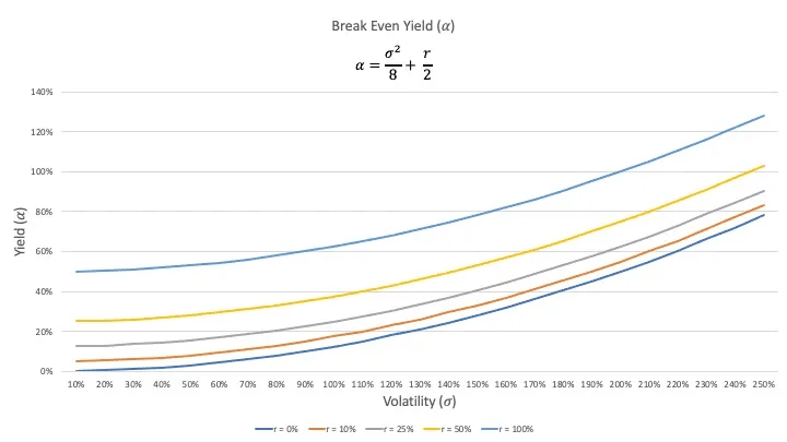
Expected Yield: Swap Rate

Assuming risk neutral pricing, we can also easily calculate the yield that would result in break even returns for liquidity providers in an UniswapV2 pool. This yield is the swap rate that a liquidity provider receives to expose herself to the expected losses from volatility.

The yield is the variance divided by 8, which is simply a cancellation term of the risk, from the risky half of the funds in the CFMM. This is in addition to half the risk free rate of return, which represents earnings from the non risky half of the funds in the CFMM that could have been invested at the risk free rate of return.

Risk Neutral Pricing vs The Real World

Given the lack of hedging options for the long tail of cryptocurrency assets, the lack of a true free floating risk free interest rate in the market place, and the fact that most market participants are risk averse rather than risk neutral, the assumption of risk neutral pricing is not a realistic assumption for the majority of risky assets.

Moreover, such an assumption would overestimate the implied volatility of many risky assets since the true drift of risky assets such as Bitcoin or Ethereum is much higher than the risk free rate of return. For example, under the capital asset pricing model, market participants add a premium for taking on risk. Therefore, risky assets such as Bitcoin or Ethereum would be expected to have higher drifts (expected returns) than the risk free rate of return.

Nevertheless, since the risk neutral pricing framework is assuming very well functioning markets (good hedges and liquidity available) with emotionally unbiased investors (risk neutral rather than risk averse), one can therefore think of it as calculating lower and upper bounds for the variables of interest to a liquidity provider in a CFMM like UniswapV2.

For example, the lowest estimate of the yield that would break even liquidity provision in a CFMM or alternatively the highest estimate of implied volatility from the CFMM given the current yield. In addition, the assumption of risk neutral pricing helps us better understand the relationships between different variables that affect the returns of liquidity provision. This knowledge can help us design more efficient functioning CFMMs.

CFMM Design

Having a better understanding of the market variables that should determine the yield in a CFMM pool, a better CFMM can be constructed to ensure lasting availability of liquidity in decentralized exchanges.

First and foremost, as you can see in the formula above, under the risk neutral assumption, the yield of the CFMM has a quadratic relationship with the volatility of the risky asset and a linear relationship with the risk free rate of return. It does not have any relationship with the trading volumes of the risky asset.

While there may be some correlation between volume and volatility, it is not necessary that the relationship be quadratic or even linear.

The correlation coefficient of ETH/USDC daily trading volume as a percentage of liquidity in UniswapV2 averaged over 30 days and the 30 day historical volatility of ETH/USDC since UniswapV2’s inception is approximately 50%.

Therefore, whatever incentive model one would create to remunerate liquidity providers for providing liquidity in a CFMM would have to be an exponential model, whose payments grows with the square of a proxy for the volatility of the risky asset. It cannot be a flat fee on trading volumes.

LVR & Trading Fees

An academic paper was recently submitted examining the profitability of automated market makers such as UniswapV2 for liquidity providers under risk neutral assumptions. In it, the running cost of liquidity provision in UniswapV2 was estimated. The authors called this number the LVR (Loss vs Rebalancing).

The LVR was calculated by first assuming the risk neutral assumption of being able to hedge the liquidity provision portfolio completely using an external exchange. Then Ito’s lemma was used to calculate the rate of change in the value of the liquidity provision portfolio with respect to price while taking into account the stochastic nature of the portfolio in a Black Scholes setting. The estimation of the LVR for UniswapV2 pools, as a percentage of the funds in the pools, was the variance of the risky asset divided by 8. Therefore, a yield equal to this number was given as the break even yield for liquidity providers in UniswapV2.

Given the 0.3% fee rate of UniswapV2 and assuming a fairly reasonable 5% daily volatility for ETH/USD, using the above formula for the break even yield, it was concluded that for UniswapV2 ETH/USDC pool liquidity providers to break even, daily trading volumes would have to be approximately 10% of the liquidity in the pool.

While the estimation of the running costs of liquidity provision with respect to price, as a percentage of liquidity, in UniswapV2, as the variance of the risky asset divided by 8 is correct, equating this estimate to the break even yield only makes sense under a zero interest rate or zero drift assumption. Assuming risk neutral investors and that the portfolio can be almost perfectly hedged, a yield that only compensates you for the losses from price variation, in a non zero interest rate environment, would create an arbitrage opportunity from the lack of returns despite the passage of time.

For example, if the yield fully compensates you only for the losses from price variation while there is a positive interest rate, then one could borrow the liquidity provision portfolio, pull out the funds, and invest those funds at the risk free rate of return. The arbitrageur would earn an arbitrage yield equivalent to the risk free rate of return.

Therefore, a calculation of the break even yield for liquidity provision must take into account the risk free rate of return as we have done in this article.

However, assuming risk neutrality, even taking into account the risk free rate of return, with the current fed funds rate at 2.5%, would still imply a break even daily trading volume of close to 10% of pool liquidity. A huge underestimation of the actual daily trading volume needed. This is because it is not realistic to expect the drift of ETH/USD to be equivalent to the risk free rate of return of 2.5% given ETH/USD’s average annual return of 200% over its entire existence. Even if one concentrates only on the past two years, the period since UniswapV2 was launched, the average annual return has been approximately 120%.

Considering the riskiness of ETH as an asset relative to traditional financial assets and its relative novelty, not only as an investment product but as a technological breakthrough, it is not unreasonable for investors to demand a substantial risk premium over the risk free rate of return. Therefore, assuming an annual drift of 100%, only half of what it has historically been, the daily trading volume as a percentage of liquidity in the pool for liquidity providers to break even would have to be approximately 42%.

Taking a look at historical trading volumes as a percentage of liquidity in UniswapV2 ETH/USDC pool, this has been far from the case.

Fee-less CFMM

A proposed solution for the issue of yields needing a quadratic relationship with volatility has been to increase the trading fee rate as volatility increases. However, this approach would make CFMMs less competitive as trading venues compared to centralized exchanges such as Binance and Coinbase who already charge lower fees than the 0.3% UniswapV2 charges with progressive rates that trend to zero as trading volume grows.

A better solution, I believe, is to charge traders zero fees and shift the cost of providing liquidity to market participants that want to take the opposite side of the trade of liquidity providers. That is, if liquidity providers want to sell volatility, they should be paid by market participants that want to buy volatility. This is something we seek to achieve with the GammaSwap protocol.

Conclusion

In this article I provided a model for calculating the value of a straddle from a CFMM such as UniswapV2 based on any strike price. That model will serve to explain how to create higher delta hedges using the GammaSwap protocol that are more cost efficient than traditional short or long hedges.

I also provided a formula to calculate the implied volatility and break even yield from an UniswapV2 CFMM under the risk neutral pricing assumption. Also I demonstrated that using trading fees from volumes to compensate liquidity providers is a poor design for a CFMM given that LPs are selling volatility and should be compensated directly by someone taking the opposite side of the trade, buying volatility.

Volume != Volatility. Rather, enabling a CFMM based on a two sided volatility marketplace, where sellers can short vol and borrowers can long vol, should scale infinitely more efficiently.