Expected Impermanent Loss in Uniswap V2 & V3

Introduction

In a previous article, I showed how to calculate impermanent loss in Uniswap V2.

In this article, I’ll show how to calculate expected impermanent loss in Uniswap V2 & V3.

To read about the derivation of the calculation of impermanent loss in Uniswap V3 you can read the paper by Jiahua Xu et al

Geometric Brownian Motion

To calculate the expected impermanent loss we will assume that asset prices move in a Geometric Brownian Motion (GBM)with lognormally distributed price returns.

where S_t is the price of the asset at time t, S_0 is the price of the asset at the initial time, σ is the volatility of the log returns of the asset, μ is the expected log return of the asset, and W_t is a Wiener process that follows a normal distribution with mean 0 and variance t.

This is a fair assumption that is typically made about asset prices in traditional asset pricing models such as the Black Scholes Model for pricing options.

Expected Impermanent Loss in Uniswap V2

First remember the formula for impermanent loss in Uniswap V2 from the previous article about impermanent loss

Under our assumption of GBM we can now model the price of the portfolio held outside of Uniswap V2 and the portfolio of assets held inside Uniswap V2 as follows

Now we proceed to calculate the expected value of the portfolio held outside of Uniswap V2, which is the same function except with the exponential resolved to the expected value of the GBM

Next we calculate the expected value of the portfolio held in Uniswap V2.

Completing the square of the exponential in the integral yields

Since the part of the integral above is a Probability Density Function (PDF), it integrates to one. Therefore, the final result for the expected value of the portfolio held in Uniswap V2 is as follows

And, the formula for the expected value of the impermanent loss is as follows

However, taking notice of the cosh identity

and setting

We can simplify the formula for the expected value of the impermanent loss to the following

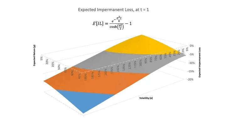
We can now create a chart of the expected impermanent loss for different values of volatility (σ)

If we chart the expected impermanent loss as a surface across volatility (σ) and mean return (μ) we get

As we can infer from the equation for expected impermanent loss as volatility (σ), expected return (μ), and time (t) go to infinity the expected impermanent loss goes to -100%. However, the effect of the expected return (μ) is greater than that of volatility (σ), since at every level of volatility the impermanent loss is significantly higher the higher the expected return or drift (μ) of the asset.

Expected Impermanent Loss in Uniswap V3

To calculate the formula for expected impermanent loss in Uniswap V3 we have to first take note of the formulas for impermanent loss in Uniswap V3

where

First notice that the formula for impermanent loss in Uniswap V3 depends on three different price ranges that are determined by the range a liquidity provider chooses to provide liquidity at. As the range picked by a liquidity provider increases, the more the impermanent loss in Uniswap V3 approaches that of Uniswap V2.

Therefore a liquidity provider that wants to estimate the expected impermanent loss of an Uniswap V3 position that is providing liquidity across a very large price range can simply use the formula for expected impermanent loss in Uniswap V2. That is the price range selected is trivial because the impermanent loss of the Uniswap V3 position will resemble that of an Uniswap V2 position.

However, if a liquidity provider is using a non trivial price range, the top and bottom range formulas become relevant. Therefore, due to our assumption of GBM, we would need to integrate the normal distribution curve over all three separate price ranges. This would result in a very complex equation, since there won’t be a single integral that resolves to one.

To avoid this we will use a computational approach to find the expected impermanent loss for Uniswap V3 liquidity pool positions that use a non trivial price range. We will therefore do a monte carlo simulation of 10,000 iterations written in python.

First we write a function to generate a random number according to a normal distribution with mean μ (mu) and standard deviation σ (sigma)

#Standard Normal variate using Box-Muller transform.
def random_bm(mu, sigma):
	u = 0
	v = 0
	while(u == 0): 
    	u = random() #Converting [0,1) to (0,1)
	while(v == 0): 
    	v = random()
	mag = sigma * math.sqrt( -2.0 * math.log( u ) )
	return mag * math.cos( 2.0 * math.pi * v ) + mu

Then we write a function to calculate the impermanent loss for an Uni V3 LP position with an arbitrary range based on the formulas for impermanent loss in Uniswap V3

def calcImpLoss(lowerLimit, upperLimit, px):
	r = math.sqrt(upperLimit/lowerLimit)
	a1 = (math.sqrt(r) - px)
	a2 = (math.sqrt(r) / (math.sqrt(r) - 1)) * (2*math.sqrt(px) - (px + 1))
	a3 = (math.sqrt(r) * px - 1)

	if(px < 1/r):
    	return a3
	elif(px > r): 
    	return a1

	return a2;

Then we write a function to perform the Monte Carlo Simulation over a large number of iterations (e.g. 10,000 iterations)

def calcExpImpLoss(rangePerc, mu, sigma) :
	upperPx = 1 + rangePerc
	lowerPx = 1 / upperPx
	Vhsum = 0
	impLossSum = 0
	iterations = 10000
	for i in range(iterations) :
    	t = 1
    	W = random_bm(0, 1) * math.sqrt(t-0)
    	X = (math.log(1 + mu) - 0.5 * math.pow(math.log(1 + sigma), 2)) * t + math.log(1 + sigma) * W
    	_px = math.exp(X)
    	Vhsum += 1 + _px
    	impLossSum += calcImpLoss(lowerPx, upperPx, _px)

	return (impLossSum/iterations)/(Vhsum/iterations)

Notice in the function above that we convert the mean return (mu) and volatility (sigma) to their natural log equivalents when using the function random_bm(). We do that because the assumption is that prices are lognormally distributed therefore we need the natural log version of the mean return and volatility to obtain the random price. We then exponentiate the Euler number to this price to obtain the actual random price.

The complete code in python is below

#!/usr/bin/env python3
import math
from random import random
#Standard Normal variate using Box-Muller transform.
def random_bm(mu, sigma):
	u = 0
	v = 0
	while(u == 0): 
        u = random() #Converting [0,1) to (0,1)
	while(v == 0): 
        v = random()
	mag = sigma * math.sqrt( -2.0 * math.log( u ) )
	return mag * math.cos( 2.0 * math.pi * v ) + mu

def calcImpLoss(lowerLimit, upperLimit, px):
	r = math.sqrt(upperLimit/lowerLimit)
	
    a1 = (math.sqrt(r) - px)
	a2 = (math.sqrt(r) / (math.sqrt(r) - 1)) * (2*math.sqrt(px) - (px + 1))
	a3 = (math.sqrt(r) * px - 1)
	if(px < 1/r):
    	return a3
	elif(px > r): 
    	return a1

	return a2;

def calcExpImpLoss(rangePerc, mu, sigma) :
	upperPx = 1 + rangePerc
	lowerPx = 1 / upperPx
	Vhsum = 0
	impLossSum = 0
	iterations = 10000
	for i in range(iterations) :
    	t = 1
    	W = random_bm(0, 1) * math.sqrt(t-0)
    	X = (math.log(1 + mu) - 0.5 * math.pow(math.log(1 + sigma), 2)) * t + math.log(1 + sigma) * W
    	_px = math.exp(X)
    	Vhsum += 1 + _px
    	impLossSum += calcImpLoss(lowerPx, upperPx, _px)

	return (impLossSum/iterations)/(Vhsum/iterations)

Conclusion

In this article I showed a formula to calculate the expected impermanent loss in Uniswap V2 and Uniswap V3.

Since Uniswap V2 and V3 are a type of options market where liquidity providers are taking short volatility positions, we can now devise a way to calculate the implied volatility of Uniswap V2 and Uniswap V3 from the current yields, which I will cover in the next article.